The Fundamental Theorem of Calculus

A close-up of concentric growth rings and radial cracks in a cut tree trunk. — Photo by Kasman on Pixabay.

An integral tells us how infinitesimal contributions combine to give an exact total. So far, we’ve evaluated integrals by recognizing familiar geometric regions, but many functions produce curves whose areas we don’t know how to calculate. How can we find these totals without relying on a convenient shape?

Differentiation gives us a way forward. If we recognize the contribution in an integral as the differential of a function, adding those small changes gives the difference between its ending and starting values. The Fundamental Theorem of Calculus makes this connection precise. In this lesson, we’ll use familiar differentiation rules to find antiderivatives and evaluate integrals. We’ll also see how a known starting value lets us use the accumulated change to find an ending value.

By the end of this lesson, you should be able to:

Use the Fundamental Theorem of Calculus to evaluate definite integrals.
Find an ending value from a known starting value and an accumulated change.
Find indefinite integrals of power functions and polynomials.

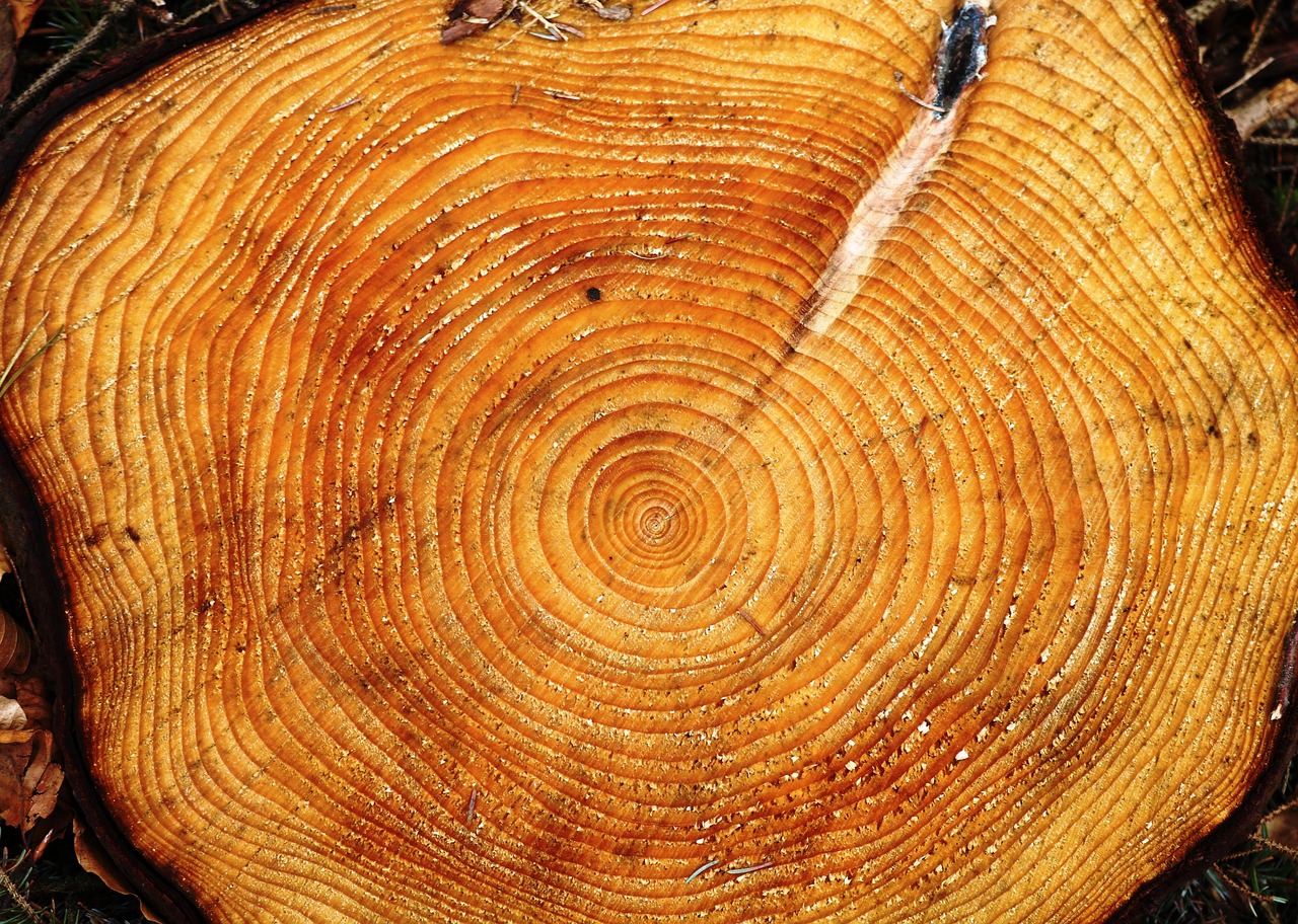
The rings in a tree trunk record growth around wood that was already there. New wood forms just beneath the bark, outside the older wood. Looking at a cross-section, how much new area is added when the trunk's radius grows from $10\,\text{cm}$ to $11\,\text{cm}$ ?

We'll model the wood's cross-section at one fixed height as a circle, setting aside the bark and the irregularities of a real trunk. At radius $10\,\text{cm}$ , its circumference is $\text{cm}$ ; at radius $11\,\text{cm}$ , it's $\text{cm}$ .

The same small increase in radius spreads new wood around the whole circumference. As the trunk gets wider, you should expect that small increase to add .

Let $$ r $$ be the radius, measured in $\text{cm}$ , and let $$ A $$ be the cross-sectional area, measured in $\text{cm}^2$ . An infinitesimal increase $\dd{r}$ adds an infinitesimal ring at the outside. An annual growth ring contains many such layers; $\dd{r}$ represents the width of one infinitesimal contribution.

Loading the graph…If it does not appear, check the Desmos API configuration.

Blue is the wood already present; red is one newly added infinitesimal layer. Cut open and laid out, the layer has length

2\pi r

and width

\dd{r}

. Its width is exaggerated so you can see it; the drawings aren't to scale.

A ring of finite thickness has a longer outer edge than inner edge; however, at an infinitesimal scale, the difference between these edges is negligible, so we can imagine "flattening" the ring into a rectangle that has a length of $2\pi r$ and a width of $\dd{r}$ . Multiplying these dimensions gives the infinitesimal area contribution:

$\dd{A}=2\pi r\dd{r}.$

Since $$ r $$ and $\dd{r}$ have units of $\text{cm}$ , the units of $\dd{A}$ must be .

The new wood lies between the original and final radii. Accumulating just those layers gives

$\text{area added}=\int_{10}^{11}2\pi r\dd{r}.$

We can find this area using geometry. Imagine cutting open all the infinitesimal rings in a disk and laying their strips next to one another, ordered from the center outward. Their lengths increase from zero to the outer circumference. Because the length $2\pi r$ increases linearly with radius, their ends form a straight sloping edge: together the strips make a triangle.

On a graph of circumference against radius, each straightened ring becomes a vertical strip of height $2\pi r$ and width $\dd{r}$ . All the strips from the center to the outer radius form the triangle under the line. The added wood corresponds to just the strips between $$ r=10 $$ and $$ r=11 $$ .

Loading the graph…If it does not appear, check the Desmos API configuration.

The red region represents

\displaystyle \int_{10}^{11}2\pi r\dd{r}

. The triangle extending to

\( r=11 \)

contains both shaded regions; subtracting the blue triangle extending to

\( r=10 \)

leaves the red region. Each vertical strip has height

2\pi r

and infinitesimal width

\dd{r}

Using the triangle-area formula, the added area is

$\frac12(22\pi)(11)-\frac12(20\pi)(10).$

According to the circular model, the new wood has area $\text{cm}^2$ .

The same construction works for any disk of radius $$ r $$ . Its straightened layers form a triangle with dimensions $$ r $$ and $2\pi r$ , so its area is

$\displaystyle \frac12(2\pi r)r=\)\(\displaystyle .$

That's the familiar circle-area formula. In our subtraction, each triangle's area is the value of $\pi r^2$ at its corresponding radius:

$\int_{10}^{11}2\pi r\dd{r}=\pi(11)^2-\pi(10)^2.$

There's a calculus connection here. Using the differentiation rules you already know, the differential of this area expression is

$\displaystyle \dd{(\pi r^2)}=\)\(\displaystyle .$

It's exactly the contribution $2\pi r\dd{r}$ inside our integral! The geometry gave us the total first; differentiating its formula recovered one infinitesimal layer. In fact, we call $\pi r^2$ an antiderivative of $2\pi r$ , because the derivative of $\pi r^2$ is $2\pi r$ .

Loading the graph…If it does not appear, check the Desmos API configuration.

The red annulus is the wood added as the radius grows from

10\,\text{cm}

11\,\text{cm}

, with modeled area

21\pi\,\text{cm}^2

. Its finite width of

1\,\text{cm}

contains the infinitesimal layers we accumulated.

We now have a more systematic way to calculate integrals. Instead of finding a geometric formula for each new accumulation, we can work backward from the contribution: find an expression whose differential matches it, then subtract the expression's starting value from its ending value. The infinitesimal changes add up to that whole change. The Fundamental Theorem of Calculus makes this connection available beyond our circle: familiar differentiation rules can become tools for calculating integrals.

Antiderivatives and definite integrals

A definite integral gives us a way to describe an exact total by adding infinitesimal contributions. Computing that total, however, is another matter. So far, familiar geometric shapes have helped us evaluate some integrals, but a curved graph may not give us a shape whose area we already know. We'd like a method that works directly with the function in the integral (the integrand).

The key is to recognize that there’s a connection between small changes and overall (“net”) change. Suppose we can recognize the integrand as the derivative of some function $$ f $$ ; then the whole contribution, including $\dd{x}$ , is the differential of that function:

$f'(x)\dd{x}=\dd{f}.$

This means that in order to compute an integral, we’ll often need to work backwards from a given derivative.

For example, $\pi r^2$ is an antiderivative of $2\pi r$ , since $\displaystyle \dv{r} \pi r^2=2\pi r$ . Its differential is $\dd{(\pi r^2)}=2\pi r\dd{r}$ .

The circle gives us a useful way to think about what an antiderivative does. Each infinitesimal ring contributes a small change in area, and adding those changes gives the final area minus the initial area.

The same reasoning applies whenever we can recognize the contribution in an integral as the differential of a function $$ f $$ . As $$ x $$ goes from $$ a $$ to $$ b $$ , adding these infinitesimal changes gives the accumulated change in $$ f $$ , or its net change. To calculate that change, we only need its ending and starting values: $$ f(b)-f(a) $$ .

An integrand usually isn't handed to us with a prime already attached. The useful step is to recognize it as the derivative of some function, or to recognize the contribution with $\dd{x}$ as that function's differential. Once we've made that connection, the theorem lets us evaluate the integral by endpoint subtraction. Increases and decreases both count, with their signs, toward the net change.

We often write the endpoint subtraction using a convenient shorthand:

$\eval{f(x)}_a^b=f(b)-f(a).$

To read this notation, substitute the upper bound $$ b $$ into the expression to the left of the bar, then subtract the value obtained by substituting the lower bound $$ a $$ . The bar saves us from writing both substitutions every time. If we reverse the bounds, we reverse the subtraction, just as we expect from the Reversal Property of integrals.

Example

Evaluate $\displaystyle \int_1^2 3x^2\dd{x}$ .

Solution

We can recognize that $\displaystyle 3x^2$ is the derivative of $\displaystyle x^3$ by the Power Rule, so $\displaystyle x^3$ is an antiderivative of $\displaystyle 3x^2$ . Thus

$\begin{aligned}\int_1^2 3x^2\dd{x}&=\eval{x^3}_1^2\\ &=2^3-1^3\\ &=7.\end{aligned}$

Loading the graph…If it does not appear, check the Desmos API configuration.

The shaded region under

\displaystyle y=3x^2

from

\displaystyle x=1

\displaystyle x=2

represents

\displaystyle \int_1^2 3x^2\dd{x}

. Its signed area is

\displaystyle 7

, equal to the change

\displaystyle 2^3-1^3

in the antiderivative

\displaystyle x^3

. The curve shown is the integrand

\displaystyle 3x^2

A quick rearrangement of the FTC gives us a way to determine an ending value using a known starting value and the accumulated change:

This becomes especially useful when an integral comes from a physical model. Once we've identified the infinitesimal contribution, the same endpoint calculation gives the total.

Example

Suppose that to stretch an elastic device by $$ x $$ meters, it takes a force of $$ F(x)=300x^2 $$ newtons. At a stretch of $0.1\,\text{m}$ , it stores $0.1\,\text{J}$ of potential energy. If all further work is stored as potential energy, with no losses, how much energy does it store at a stretch of $0.2\,\text{m}$ ?

Solution

Let $\displaystyle E(x)$ be the stored potential energy. For an infinitesimal displacement $\displaystyle \dd{x}$ , the added work gives an energy contribution $\displaystyle \dd{E}=F(x)\dd{x}$ . Adding these contributions from $\displaystyle x=0.1$ to $\displaystyle x=0.2$ gives the accumulated change in energy.

Loading the graph…If it does not appear, check the Desmos API configuration.

The region under

\displaystyle F(x)=300x^2

from

\displaystyle x=0.1

\displaystyle x=0.2

represents the added work, equal to the increase in stored energy. A red strip of height

\displaystyle F(x)

and infinitesimal width

\displaystyle \dd{x}

represents one contribution

\displaystyle F(x)\dd{x}

; its width is exaggerated to make it visible. Force in newtons times displacement in meters gives work in joules.

To evaluate the integral, we need an antiderivative of $\displaystyle 300x^2$ . We know that differentiating $\displaystyle x^3$ gives $\displaystyle 3x^2$ , so multiplying $\displaystyle x^3$ by $\displaystyle 100$ gives the coefficient we need. The Fundamental Theorem of Calculus now gives

$\begin{aligned}E(0.2)-E(0.1)&=\int_{0.1}^{0.2}300x^2\dd{x}\\ &=\eval{100x^3}_{0.1}^{0.2}\\ &=0.8-0.1\\ &=0.7\,\text{J}.\end{aligned}$

The integral gives the added energy. Combining it with the given starting energy gives $E(0.2)=0.1+0.7=0.8\,\text{J}\text.$

Indefinite integrals and the Anti-Power Rule

When we evaluated $\displaystyle \int_1^2 3x^2\dd{x}$ , we used $$ x^3 $$ as our antiderivative. But notice that we've been careful to say that $$ x^3 $$ is an antiderivative, not the antiderivative. This is because a given function has multiple possible antiderivatives — for example, $$ x^3+5 $$ is another antiderivative of $$ 3x^2 $$ , since its derivative is also $$ 3x^2 $$ .

It's often useful to describe all the antiderivatives at once. If $$ f $$ is one antiderivative, then $$ f+C $$ has the same derivative for any constant $$ C $$ , because differentiating the added constant gives zero. If two functions have the same derivative, their difference has derivative zero, so that difference must be constant. Visually, adding a constant to any function has the effect of vertically shifting every value by the same amount. It therefore shifts both endpoint values equally, leaving their difference — and hence the slope — unchanged.

Loading the graph…If it does not appear, check the Desmos API configuration.

The graphs of

\( x^3 \)

\( x^3+3 \)

, and

\( x^3-3 \)

all have derivative

\( 3x^2 \)

. Their heights differ, but each rises by

\( 7 \)

between

\( x=1 \)

and

\( x=2 \)

. Shifting a graph vertically changes its heights without changing this rise.

When we want to describe the whole family of antiderivatives of a function, we use the integral symbol without lower and upper bounds.

Notice that we should expect a different kind of answer for definite versus indefinite integrals:

With a definite integral $\displaystyle \int_a^b f'(x)\dd{x}$ , we want a signed total over a specified interval, so the answer is a single value.
With an indefinite integral $\displaystyle \int f'(x)\dd{x}$ , we want the family of antiderivatives, so the answer includes an arbitrary constant. The constant $$ C $$ accounts for all the possible vertical shifts.

Finding an antiderivative was fairly quick when the integrand was $$ 3x^2 $$ . What if it were just $$ x^2 $$ , or a fractional or negative power? Rather than guessing each time, we can reverse engineer the Power Rule to work out a general pattern.

When we used the Power Rule, we multiplied by the exponent and then subtracted one from the exponent. To reverse engineer that process, we do the opposite things in the opposite order: first add one to the exponent, then divide by the exponent we've just recovered. For example, suppose we want an antiderivative of $$ x^2 $$ . We first add one to get an exponent of $$ 3 $$ , then divide by $$ 3 $$ , giving us $\displaystyle \frac{x^3}{3}$ . We can check our result by taking the derivative, which indeed gives us the $$ x^2 $$ we started with.

We'll generalize this process below.

Example

Find $\displaystyle \int x^2\dd{x}$ , $\displaystyle \int\sqrt{x}\dd{x}$ , and $\displaystyle \int\frac1{x^2}\dd{x}$ .

Solution

For $\displaystyle x^2$ , the new exponent is $\displaystyle 3$ . Dividing by $\displaystyle 3$ compensates for the factor that differentiation will introduce:

$\int x^2\dd{x}=\frac{x^3}{3}+C\text.$

For the square root, first write $\displaystyle \sqrt{x}$ as $\displaystyle x^{1/2}$ . This puts the integrand in the form the rule uses. Adding one to $\displaystyle 1/2$ gives $\displaystyle 3/2$ , so

$\begin{aligned}\int x^{1/2}\dd{x}&=\frac{x^{3/2}}{3/2}+C\\ &=\frac23x^{3/2}+C\text.\end{aligned}$

For $\displaystyle 1/x^2$ , first rewrite the integrand as $\displaystyle x^{-2}$ . Adding one to the exponent gives $\displaystyle -1$ . We divide by that new exponent just as before:

$\begin{aligned}\int\frac1{x^2}\dd{x}&=\int x^{-2}\dd{x}\\ &=\frac{x^{-1}}{-1}+C\\ &=-x^{-1}+C\text.\end{aligned}$

We can check each of these by differentiating.

Combining antiderivatives

Most of the integrals we want to evaluate involve more than a single power. A density, for example, might have a constant part and a part that varies with position. If we can find an antiderivative of each part, how should we combine them?

These rules come straight from the corresponding rules for derivatives and differentials. Adding or subtracting functions adds or subtracts their derivatives, so the same operations combine their antiderivatives. Multiplying by a constant $$ k $$ scales the differential.

Together, these rules and the Anti-Power Rule let us evaluate integrals of polynomials.

Rewriting roots as powers lets us use the same rules in other integrals.

Example

A rod is $4\,\text{m}$ long. At a point $$ x $$ meters from one end, its linear mass density (mass per unit length) is $\rho(x)=(3+2\sqrt{x})\,\text{kg}/\text{m,}\qquad 0\le x\le4\text.$ Find the mass of the rod.

Solution

An infinitesimal piece of length $\displaystyle \dd{x}$ has mass $\displaystyle \dd{M}=\rho(x)\dd{x}$ . Multiplying density in kilograms per meter by length in meters gives mass in kilograms. Adding the pieces from $\displaystyle x=0$ to $\displaystyle x=4$ gives the whole mass.

Loading the graph…If it does not appear, check the Desmos API configuration.

The region under

\displaystyle \rho(x)=3+2\sqrt{x}

from

\displaystyle x=0

\displaystyle x=4

represents the mass. Blue shows the constant density contribution of

\displaystyle 3

; green shows the additional contribution from

\displaystyle 2\sqrt{x}

. A red strip of height

\displaystyle \rho(x)

and infinitesimal width

\displaystyle \dd{x}

represents mass

\displaystyle \rho(x)\dd{x}

. Its width is exaggerated to make it visible.

We rewrite $\displaystyle \sqrt{x}=x^{1/2}$ , then combine antiderivatives of the constant and power terms:

$\begin{aligned}M&=\int_0^4(3+2x^{1/2})\dd{x}\\ &=\eval{3x+\frac{2x^{3/2}}{3/2}}_0^4\\ &=\eval{3x+\frac43 x^{3/2}}_0^4\\ &=12+\frac{32}{3}\\ &=\frac{68}{3}\,\text{kg}.\end{aligned}$

The constant density contributes $\displaystyle 12\,\text{kg}$ , and the square-root part contributes $\displaystyle \frac{32}{3}\,\text{kg}$ . These add to the rod's total mass, just as the blue and green regions add to the whole region under the graph.

The Fundamental Theorem of Calculus thus gives us a new way to evaluate an integral: recognize the contribution as a differential, then find the overall change in the corresponding function. For the functions we have worked with here, the Anti-Power Rule and the rules for combining antiderivatives give us a practical way to do this, although sometimes a little algebra is needed first to put the integrand into a useful form. And we can always check a proposed antiderivative by differentiating it; once it checks out, evaluating at the bounds and subtracting gives the total we were looking for.

Evaluate the following indefinite integrals. All of them can use the Anti-Power Rule, though you may need to do some algebra first.
1. $\displaystyle \int ${integrand}\dd{x}=$ .
  
  Solution
  Add one to the exponent, then divide by the new exponent: $\displaystyle ${antiderivative}+C$ . Differentiation returns $\displaystyle ${integrand}$ .
2. $\displaystyle \int ${integrand}\dd{x}=$ .
  
  Solution
  The constant coefficient stays as a factor while the Anti-Power Rule gives $\displaystyle ${antiderivative}+C$ .
3. $\displaystyle \int(${polynomial_integrand})\dd{x}=$ .
  
  Solution
  
  Integrate each term and combine the constants:
  
  $${polynomial_antiderivative}+C.$
  
  Differentiation returns all three original terms, including the negative middle term.
4. $\displaystyle \int ${integrand}\dd{x}=$ .
  
  Solution
  Rewrite the integrand as $\displaystyle ${power_factor}^{1/2}$ . The Anti-Power Rule gives $\displaystyle ${antiderivative}+C$ .
5. $\displaystyle \int\frac{${k}}{x^{${n}}}\dd{x}=$ .
  
  Solution
  The integrand is $\displaystyle ${power_factor}^{-${n}}$ . Adding one to the exponent and dividing by it gives $\displaystyle ${antiderivative}+C$ . Differentiation cancels the two minus signs.
6. $\displaystyle \int\frac{${k}}{\sqrt{x}}\dd{x}=$ .
  
  Solution
  Write the integrand as $\displaystyle ${power_factor}^{-1/2}$ . Add one to obtain $\displaystyle 1/2$ , then divide by $\displaystyle 1/2$ : $\displaystyle ${antiderivative}+C$ .
7. $\displaystyle \int(${first_factor})(${second_factor})\dd{x}=$ .
  
  Solution
  
  Expand the product first: $(${first_factor})(${second_factor})=${expanded}.$
  
  Now apply the Sum/Difference and Constant Multiple Rules:
  
  $\int(${expanded})\dd{x}=${antiderivative}+C.$
  
  Multiplying antiderivatives of the two factors would not give this answer. Differentiating such a product uses the Product Rule, producing extra terms.
8. $\displaystyle \int\frac{${numerator}}{x^2}\dd{x}=$ .
  
  Solution
  Dividing each numerator term by $\displaystyle x^2$ gives $\displaystyle ${rewritten}$ . Integrate term by term to obtain $\displaystyle ${antiderivative}+C$ .
Evaluate the following definite integrals.
1. $\displaystyle \int_0^{${b}} ${integrand}\dd{x}=$ .
  
  Solution
  $\displaystyle \eval{${antiderivative}}_0^{${b}}=${z}-0=${z}$ .
2. $\displaystyle \int_{${start}}^{${end}}(${integrand})\dd{x}=$ .
  
  Solution
  
  $\begin{aligned}\int_{${start}}^{${end}}(${integrand})\dd{x}&=\eval{${antiderivative}}_{${start}}^{${end}}\\&=${end_value}-${start_value}\\&=${z}.\end{aligned}$
  
  The ending bound is smaller than the starting bound. Since the integrand is positive, this right-to-left integral is negative.
3. $\displaystyle \int_1^4\frac{${numerator}}{\sqrt{x}}\dd{x}=$ .
  
  Solution
  
  For constants $\displaystyle a$ and $\displaystyle b$ , dividing each numerator term by $\displaystyle \sqrt{x}=x^{1/2}$ gives $\frac{ax+b}{\sqrt{x}}=ax^{1/2}+bx^{-1/2}\text.$ For the coefficients here, combining the two Anti-Power antiderivatives gives $\displaystyle ${antiderivative}$ .
  
  $\begin{aligned}\int_1^4\frac{${numerator}}{\sqrt{x}}\dd{x}&=\eval{${antiderivative}}_1^4\\&=(${upper_value})-(${lower_value})\\&=${z}.\end{aligned}$
A circular trunk grows from radius $${a}\,\text{cm}$ to radius $${b}\,\text{cm}$ .
1. Explain why an infinitesimal layer contributes $2\pi r\dd{r}$ to area, and write the integral for the added area.
  
  Solution
  The circumference is $\displaystyle 2\pi r$ and the infinitesimal thickness is $\displaystyle \dd{r}$ . Their product is the layer's area. Adding only the new layers gives $\displaystyle \int_{${a}}^{${b}}2\pi r\dd{r}$ .
2. The added area is $\text{cm}^2$ .
  
  Solution
  
  An antiderivative is $\displaystyle \pi r^2$ , so
  
  $\begin{aligned}\int_{${a}}^{${b}}2\pi r\dd{r}&=\eval{\pi r^2}_{${a}}^{${b}}\\&=(${b}^2-${a}^2)\pi\\&=${d}\pi\,\text{cm}^2.\end{aligned}$
  
  Loading the graph…If it does not appear, check the Desmos API configuration.
  
  Radii are measured in $\displaystyle \text{cm}$ . The shaded annulus contains the new layers; the original disk is excluded.
A rod is $${b}\,\text{cm}$ long. At a point $$ x $$ centimeters from one end its density is $\rho(x)=${a}+${3*k}x^2$ grams per centimeter.
1. Write the infinitesimal mass contribution and the integral for the rod's total mass.
  
  Solution
  $\displaystyle \dd{M}=\rho(x)\dd{x}$ , so $\displaystyle M=\int_0^{${b}}(${a}+${3*k}x^2)\dd{x}$ . Density times length gives mass.
2. The mass is $\text{g}$ .
  
  Solution
  
  $\begin{aligned}M&=\eval{${rod_antiderivative}}_0^{${b}}\\&=${a}(${b})+${k}(${b})^3\\&=${z}\,\text{g}.\end{aligned}$
  
  Loading the graph…If it does not appear, check the Desmos API configuration.
  
  The height is density and the width is length, so the shaded contributions add to mass in $\displaystyle \text{g}$ .
To stretch an elastic device by $$ x $$ meters takes a force of $F(x)=${3*k}x^2$ newtons. Find the work required to stretch it from $$ 0 $$ to $1\,\text{m}$ , then from $1\,\text{m}$ to $2\,\text{m}$ .

The first stretch requires $\text{J}$ ; the second requires $\text{J}$ . The stretch requires more work. Explain why.

Solution

Each piece contributes $\displaystyle F(x)\dd{x}$ . An antiderivative is $\displaystyle ${work_antiderivative}$ . The first stretch requires $\displaystyle \eval{${work_antiderivative}}_0^1=${k}\,\text{J}$ ; the second requires $\displaystyle \eval{${work_antiderivative}}_1^2=${7*k}\,\text{J}$ . The second requires seven times as much work: the same stretch occurs where the force is larger.

Loading the graph…If it does not appear, check the Desmos API configuration.

Blue represents $\displaystyle ${k}\,\text{J}$ of work during the first stretch; red represents $\displaystyle ${7*k}\,\text{J}$ during the second. The widths are equal, but the second region has larger force contributions.
The graph shows $$ f' $$ , and $$ f(1)=4 $$ .

Loading the graph…If it does not appear, check the Desmos API configuration.

The marked points give values of $$ f' $$ . The two shaded triangles contribute signed area: positive above the axis and negative below it.
1. The net change is $\displaystyle f(3)-f(1)=\int_1^3 f'(x)\dd{x}=$ .
  
  Solution
  The triangle above the axis has area $\displaystyle \frac12(1)(2)=1$ . The triangle below has area $\displaystyle \frac12(1)(4)=2$ , contributing $\displaystyle -2$ . Thus $\displaystyle \int_1^3 f'(x)\dd{x}=1-2=-1$ .
2. The ending value is $$ f(3)= $$ .
  
  Solution
  The integral gives the change in $\displaystyle f$ , so we add it to the given starting value: $f(3)=f(1)+\int_1^3 f'(x)\dd{x}=4-1=3\text.$
Suppose $\displaystyle \int_0^5 f(x)\dd{x}=${p}$ and $\displaystyle \int_0^5 g(x)\dd{x}=${q}$ . Then $\displaystyle \int_0^5[${k}f(x)-g(x)]\dd{x}=$ .

Solution
The Constant Multiple and Difference Rules give $\displaystyle ${k}(${p})-${q}=${z}$ . No formulas for $\displaystyle f$ and $\displaystyle g$ are needed.