Properties of integrals

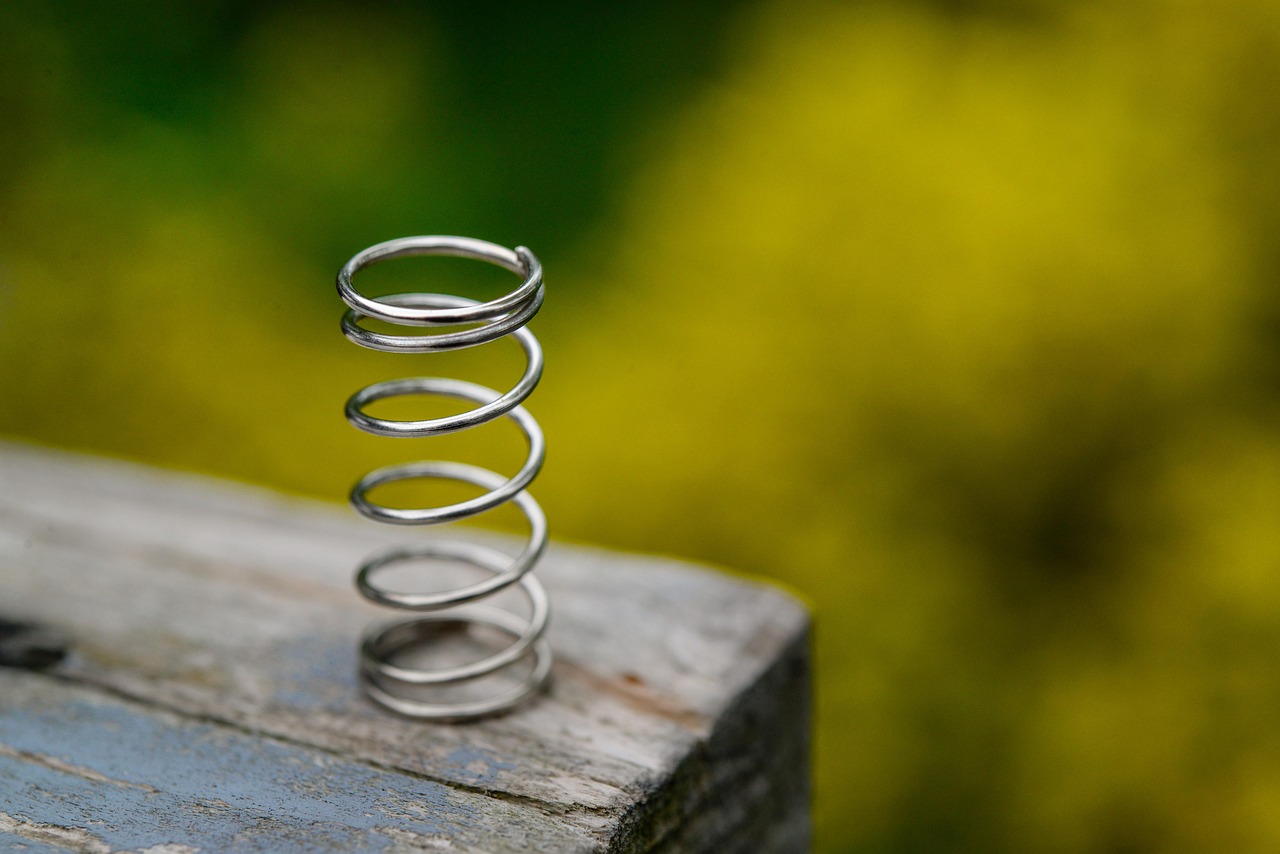
A single steel coil spring stands upright on a wooden surface. — Photo by ClickerHappy on Pixabay.

An integral gathers many small contributions into one total, but those contributions need not all have the same sign. A force can transfer energy into one object while taking it from another, and a function can lie above the horizontal axis on one part of an interval and below it on another. What should the integral tell us when some contributions oppose others?

Signed area lets the integral preserve this directional information while still producing a single net result. Once we keep track of where an accumulation starts and ends, we can also understand how adjacent intervals combine, why an interval with no length contributes nothing, and why reversing the bounds reverses the sign.

By the end of this lesson, you should be able to:

Interpret definite integrals as signed accumulations in graphical and physical contexts, including energy transfer.
Distinguish signed area from total geometric area and evaluate integrals using familiar geometric regions.
Use the Additive Interval, Zero Interval, and Reversal Properties to split and relate integrals with different bounds.

The concept of energy gives us a way to account for what happens during a physical interaction. As objects interact, energy can transfer from one to another in many different forms. Following these transfers helps us make sense of physical phenomena that might otherwise seem unrelated.

We'll follow one such transfer from beginning to end. Suppose a cart starts at rest on a frictionless track, and you push it to get it moving. With no friction to remove the energy, the cart speeds up as you push.

When a constant force points in the direction of motion, the energy transferred to the cart ( $\Delta E$ ) is the force $$ F $$ times the displacement $\Delta x$ :

$\Delta E=F\cdot\Delta x.$

So if you push with a constant force of $10\text{ N}$ (newtons) over a distance of $0.4\text{ m}$ , your push increases the cart's kinetic energy by $\text{ J}$ . (A joule is equal to one newton-meter, that is, the amount of energy gained by applying a $1\text{ N}$ force over a distance of $1\text{ m}$ .) When you stop pushing, the cart continues down the track carrying those $4\text{ J}$ of kinetic energy.

Now suppose the cart meets a relaxed spring and begins compressing it, as in the figure below. Let $$ x $$ be the displacement of the cart in meters as it compresses the spring, measured inward from the spring's relaxed position. The farther the cart moves, the more strongly it pushes on the spring. This relationship between force and displacement is linear, with the force on the spring given by $F(x)=50x\text{ N}$ . As the compression increases, this force .

Loading the graph…If it does not appear, check the Desmos API configuration.

The cart moves toward the wall, compressing the spring until it comes to rest.

Loading the graph…If it does not appear, check the Desmos API configuration.

The shaded region shows the energy transferred into the spring. The narrow purple strip marks one additional contribution.

You can use the slider to follow the cart from first contact at $$ x=0 $$ until it stops at $x=0.4\text{ m}$ . The graph beside it records the force on the spring and shades the energy transferred into it.

—

In the previous lesson, we accumulated a changing density by adding infinitesimal pieces. It turns out that the same idea applies here: each small increase in compression adds a narrow strip with height $$ F(x) $$ , so when its width is $\dd{x}$ , the strip contributes $\text{ J}$ .

During the forward motion, $\dd{x}$ is positive and the cart's force on the spring is $50x\text{ N}$ . The spring should therefore energy, and the complete amount of energy transferred should be

$\Delta E\tsub{spring}=\int_0^{0.4}50x\dd{x}\text.$

The integral is the area of the completed triangle on the force graph. Its base is $0.4\text{ m}$ and its height is $20\text{ N}$ , so its area is $\text{ J}$ . Hence the spring has gained $4\text{ J}$ of potential energy, stored because the spring is compressed.

Now let's look at the problem from the cart's perspective. While the cart pushes inward on the spring, the spring pushes outward on the cart with a force of equal magnitude. The spring's force on the cart is therefore $\text{N}$ , so the cart should energy.

In this idealized setup, energy is conserved, so the amount of kinetic energy lost by the cart should be the amount of potential energy gained by the spring.

Loading the graph…If it does not appear, check the Desmos API configuration.

The red triangle represents the spring's outward force on the cart during compression.

As before, we can represent the cart's change in kinetic energy with an integral. On the graph, the triangle lies below the $$ x $$ -axis, so we'll count its area as negative. That sign matches what's happening physically: the cart is losing energy. Its change in kinetic energy is therefore

$\displaystyle \Delta E\tsub{cart}=\int_0^{0.4}-50x\dd{x}= \)\(\displaystyle \text{ J}.$

This explains why the cart is momentarily at rest when the compression reaches $0.4\text{ m}$ : the cart has lost all its kinetic energy, which was gained by the spring as potential energy.

At maximum compression, the cart is still, but the spring isn't finished with it yet. The spring pushes the cart outward, reversing the motion.

The force on the spring is still $\text{N}$ , but the return motion makes $\dd{x}$ negative. The spring should potential energy, so its change should be equal to

$\displaystyle \Delta E\tsub{spring}=\int_{0.4}^{0}50x\dd{x}= \)\(\displaystyle \text{ J}.$

The same return motion transfers energy into the cart. The spring's force on the cart remains $\text{N}$ , and the bounds now run from $0.4\text{ m}$ back to $$ 0 $$ . The cart should kinetic energy, with a change of

$\displaystyle \Delta E\tsub{cart}=\int_{0.4}^{0}-50x\dd{x}= \)\(\displaystyle \text{ J}.$

Both directional signs are negative: the spring's force points outward, and the cart moves outward. Their product is positive. When the spring returns to its relaxed position, the cart has regained $4\text{ J}$ of kinetic energy and moves away in the opposite direction.

Throughout this investigation, energy has moved from you to the cart, from the cart to the spring, and then from the spring back to the cart. When energy is transferred by a force as an object moves over some distance, physicists call this quantity work. The magnitude of the work tells us how much energy is transferred, and the sign tells us whether energy is gained or lost.

Signed area

The quantities we accumulate don't always stay positive. Their signs often distinguish two directions or two opposing effects, so a negative value can carry meaningful information about how the total is changing. Positive contributions increase the net accumulation, while negative contributions decrease it.

Explore gave us one example: a negative force pointed opposite our chosen positive direction. In other settings, a negative velocity can describe motion in the negative direction, a negative net flow rate can describe water leaving a tank, and negative power can describe a battery sending energy out rather than receiving it. None of these represents an impossible negative amount; each sign tells us how that contribution affects the whole.

Loading the graph…If it does not appear, check the Desmos API configuration.

Only the shaded interval is included. Within those bounds, blue regions contribute positively and red regions contribute negatively.

To turn these contributions into a total, we still add them across the interval. The only new feature is that their signs now matter. When $$ a<b $$ , the increments $\dd{x}$ point from left to right, so the graph represents the integral as signed area:

$\int_a^b f(x)\dd{x}=\mathhlblue{\text{area above the axis}}-\mathhlred{\text{area below the axis}}.$

The geometric areas themselves are nonnegative; their positions relative to the axis determine their signs in the integral. A region below the axis is not somehow a negative geometric shape. Instead, its location tells us that the quantities being accumulated are negative there, so that region decreases the net total.

If we want the total geometric area instead, we count every region positively. Signed area answers a different question: it gives the net effect after opposing contributions cancel. In a physical setting, that distinction lets the integral record not only how much is transferred, but also the direction of the transfer.

Example

An elastic exercise band is anchored to a wall. As a person slowly moves its handle outward, let $$ x $$ be its distance from the relaxed position. The person pulls on the band with force $60x\text{ N}$ , while the band pulls back on the person with force $-60x\text{ N}$ , where $$ x $$ is measured in meters.

When the handle reaches $x=0.3\text{ m}$ , how much energy is stored in the band? How much energy has the person lost?

Solution

We can describe the same stretch from two perspectives. The person's force points in the direction the handle moves, so the band receives positive energy contributions. In the first panel, those contributions accumulate from left to right as the stretch increases.

Loading the graph…If it does not appear, check the Desmos API configuration.

As the band stretches, its positive energy change accumulates from left to right.

Loading the graph…If it does not appear, check the Desmos API configuration.

During the same left-to-right motion, the person's negative energy change accumulates below the axis.

The second panel follows the same left-to-right motion, but now we use the band's force on the person. That force points opposite the motion, so its contributions lie below the axis. The two triangles have the same base, $0.3\text{ m}$ , and the same height, $18\text{ N}$ ; only their signs differ.

Energy transferred by a force over a displacement is work. For the band, the positive triangle gives

$\begin{aligned}\Delta E\tsub{band}&=\int_0^{0.3}60x\dd{x}\\ &=\frac12(0.3)(18)\\ &=2.7\text{ J}.\end{aligned}$

The band stores $2.7\text{ J}$ of potential energy. For the person, the equal-sized triangle lies below the axis, so the same calculation carries a negative sign:

$\begin{aligned}\Delta E\tsub{person}&=\int_0^{0.3}-60x\dd{x}\\ &=-\frac12(0.3)(18)\\ &=-2.7\text{ J}.\end{aligned}$

The negative change says that the person loses $2.7\text{ J}$ of energy, exactly the amount stored in the band.

Adjacent intervals

An accumulation can be assembled in stages. We begin with the most intuitive arrangement: $$ b $$ lies between $$ a $$ and $$ c $$ . In the graph below, the area from $$ a $$ to $$ c $$ is divided at $$ b $$ . The blue region and purple region are adjacent; they don't overlap, and together they fill the entire region.

Loading the graph…If it does not appear, check the Desmos API configuration.

The blue region represents

\displaystyle \int_a^b f(x)\dd{x}

, and the purple region represents

\displaystyle \int_b^c f(x)\dd{x}

Accumulating from $$ a $$ to $$ b $$ and then from $$ b $$ to $$ c $$ therefore includes each contribution from $$ a $$ to $$ c $$ exactly once. It is the integral version of completing a journey in two stages.

The picture uses positive regions, but the property also works when part of the graph lies below the axis: the signed contribution of each piece is still included exactly once. We can therefore break a difficult integral into pieces that are easier to understand or calculate, then add their values.

Example

Let

$\begin{aligned}f(x)=\begin{cases}x+3,&-5\le x\le0,\\ \sqrt{9-x^2},&0\le x\le3.\end{cases}\end{aligned}$

Use the graph and the Additive Interval Property to find $\displaystyle \int_{-5}^{3}f(x)\dd{x}$ .

Loading the graph…If it does not appear, check the Desmos API configuration.

The red region is the negative triangle, the blue region is the positive triangle, and the purple region is the quarter circle.

Solution

The line crosses the axis at $$ x=-3 $$ , and its endpoint at $$ x=0 $$ is where the quarter circle begins. Splitting at both inputs gives

$\int_{-5}^{3}f(x)\dd{x}=\mathhlred{\int_{-5}^{-3}f(x)\dd{x}}+\mathhlblue{\int_{-3}^{0}f(x)\dd{x}}+\mathhlviolet{\int_{0}^{3}f(x)\dd{x}}.$

The first triangle has base and height $$ 2 $$ , but it lies below the axis and contributes $\mathhlred{-2}$ . The second triangle has base and height $$ 3 $$ , so it contributes $\mathhlblue{\frac92}$ . The final region is one quarter of a circle with radius $$ 3 $$ , contributing $\mathhlviolet{\frac{9\pi}{4}}$ . Therefore,

$\begin{aligned}\int_{-5}^{3}f(x)\dd{x}&=\mathhlred{-2}+\mathhlblue{\frac92}+\mathhlviolet{\frac{9\pi}{4}}\\ &=\frac52+\frac{9\pi}{4}\\ &\approx 9.57.\end{aligned}$

So far, we have used the Additive Interval Property in the situation suggested by the picture, with $$ b $$ between $$ a $$ and $$ c $$ . Now we can hold onto that same property and push past the original assumption. What should happen if two endpoints coincide, or if part of the journey runs backward?

The resulting rules are not extra conventions pasted onto the integral. They follow from the Additive Interval Property, and they match the physical intuition we have already developed about accumulation. First, if an accumulation begins and ends at the same input, there is no interval across which contributions can accumulate.

Next, consider a trip from $$ a $$ to $$ b $$ followed by the same trip in reverse. Together, the two stages return to the starting point, so their net accumulation must be zero. Whatever the forward trip contributed, the reverse trip must undo.

The reversal rule agrees with changing the sign of every input increment, but it also has the more direct interpretation we just saw: reversing a transfer reverses its effect. This is why the Additive Interval Property remains consistent even when the endpoints are not in increasing order. Any portion traveled in both directions contributes once with each sign and cancels.

The words “lower” and “upper” describe where the bounds are written beside the integral sign, not which number is smaller. The lower bound tells us where the accumulation starts, and the upper bound tells us where it ends. Reading the bounds as a journey keeps that order—and the sign it produces—straight.

Example

In chemistry, the specific heat of a material tells us how much energy is needed to raise the temperature of $1\text{ kg}$ of that material by $1^\circ\text{C}$ . Specific heat can vary with temperature.

Consider a $1\text{ kg}$ block of aluminum. For this particular block, let $$ C(T) $$ be its heat capacity: the energy needed to raise the entire block's temperature by $1^\circ\text{C}$ . The block's mass is already built into $$ C(T) $$ , so a simplified linear model is

$C(T)=0.8875+0.0005T\quad\frac{\text{kJ}}{{}^\circ\text{C}},$

where $$ T $$ is measured in degrees Celsius. How much energy does the block gain as its temperature rises from $25^\circ\text{C}$ to $225^\circ\text{C}$ ? What is its energy change when it later cools from $225^\circ\text{C}$ back to $25^\circ\text{C}$ ?

Solution

A small temperature increase $\dd{T}$ requires approximately $C(T)\dd{T}$ kilojoules, so adding those contributions across the temperature interval gives the block's change in energy. Heating moves forward through the interval, while cooling later moves through the same interval backward. The two graphs show the same trapezoid accumulated in opposite directions.

Loading the graph…If it does not appear, check the Desmos API configuration.

As the aluminum heats, the blue accumulation fills the trapezoid from left to right.

Loading the graph…If it does not appear, check the Desmos API configuration.

As the aluminum cools, the red accumulation fills the same trapezoid from right to left.

At the two temperatures, the line has heights $C(25)=0.9\frac{\text{kJ}}{{}^\circ\text{C}}$ and $C(225)=1\frac{\text{kJ}}{{}^\circ\text{C}}$ . Once the blue animation has filled the interval, its region is a trapezoid. We can find that area in two useful ways.

First, split it into a rectangle and a triangle. The rectangle has width $200^\circ\text{C}$ and height $0.9\frac{\text{kJ}}{{}^\circ\text{C}}$ , while the triangle has the same width and height $0.1\frac{\text{kJ}}{{}^\circ\text{C}}$ . Therefore,

$\begin{aligned}\Delta E&=\int_{25}^{225}C(T)\dd{T}\\ &=(200)(0.9)+\frac12(200)(0.1)\\ &=180+10\\ &=190\text{ kJ}.\end{aligned}$

Alternatively, use the trapezoid area formula. Its parallel bases are the two vertical sides, with lengths $0.9\frac{\text{kJ}}{{}^\circ\text{C}}$ and $1\frac{\text{kJ}}{{}^\circ\text{C}}$ , and the distance between them is $200^\circ\text{C}$ :

$\begin{aligned}\Delta E&=\frac12(0.9+1)(200)\\ &=190\text{ kJ}.\end{aligned}$

Both decompositions measure the same region, so they give the same energy change. The first makes the two familiar shapes visible; the second treats the region as a single trapezoid.

When the block cools, the function $$ C(T) $$ is still positive, but the bounds reverse because temperature now moves from $225^\circ\text{C}$ down to $25^\circ\text{C}$ . By the Reversal Property,

$\begin{aligned}\Delta E&=\int_{225}^{25}C(T)\dd{T}\\ &=-\int_{25}^{225}C(T)\dd{T}\\ &=-190\text{ kJ}.\end{aligned}$

The sign reversal has a physical meaning: the block gains $190\text{ kJ}$ while heating and loses $190\text{ kJ}$ while returning through the same temperatures. The material and the geometric region have not changed; only the direction of the transfer has.

A person slowly stretches a spring from its relaxed position. When the spring has been stretched $$ x $$ meters, the person must pull on it with force $F(x)=${spring_constant}x\text{ N}$ . Assume no energy is lost to friction or heating.
1. Sketch the graph of the person's force on the spring for $0\le x\le${stretch_label}$ . Shade the region whose signed area represents the energy transferred to the spring.
  
  Solution
  
  The force increases linearly from $0\text{ N}$ to $${end_force}\text{ N}$ . The shaded region is therefore a triangle above the horizontal axis.
  
  Loading the graph…If it does not appear, check the Desmos API configuration.
  
  The triangle under the force graph represents the energy transferred to the spring.
2. As the person stretches the spring from $$ x=0 $$ to $x=${stretch_label}\text{ m}$ , the work done by the person's force on the spring is $\text{J}$ . Energy is transferred .
  
  Solution
  
  The triangular region has base $${stretch_label}\text{ m}$ and height $${end_force}\text{ N}$ , so
  
  $\begin{aligned}\Delta E\tsub{spring}&=\int_0^{${stretch}}${spring_constant}x\dd{x}\\ &=\frac12(${stretch_label})(${end_force})\\ &=${spring_energy}\text{ J}.\end{aligned}$
  
  The positive value means that the person's work transfers $${spring_energy}\text{ J}$ into the spring, increasing its stored energy by that amount.
3. The person then keeps hold of the spring and slowly lets it return from $x=${stretch_label}\text{ m}$ to $$ x=0 $$ . The work done by the person's force on the spring is $\text{J}$ . Energy is transferred .
  
  Solution
  
  The force function is unchanged, but the motion traverses the interval in reverse. The Reversal Property gives
  
  $\begin{aligned}\Delta E\tsub{spring}&=\int_{${stretch}}^0${spring_constant}x\dd{x}\\ &=-\int_0^{${stretch}}${spring_constant}x\dd{x}\\ &=${return_energy}\text{ J}.\end{aligned}$
  
  The negative change means that $${spring_energy}\text{ J}$ leaves the spring as its stored energy decreases.
A uniform rope is $${rope_length}\text{ m}$ long and weighs $${rope_weight}\text{ N}$ . It hangs vertically from the edge of a platform. A person slowly pulls the rope straight upward, placing each retrieved part on the platform. Let $$ x $$ be the length of rope, in meters, that has already been pulled up. Ignore friction.

Loading the graph…If it does not appear, check the Desmos API configuration.

As less rope remains hanging, the required upward force decreases.
1. After $$ x $$ meters have been pulled up, the fraction of the rope still hanging is . The required force is therefore $$ F(x)= $$ $\text{N}$ .
  
  Solution
  
  The hanging length is $${rope_length}-x$ meters, so the fraction still hanging is $(${rope_length}-x)/${rope_length}$ . Multiplying that fraction by the rope's total weight gives
  
  $F(x)=${rope_weight}\left(\frac{${rope_length}-x}{${rope_length}}\right)\text{ N}.$
  
  This agrees with the graph: the required force begins at the full weight, $${rope_weight}\text{ N}$ , and decreases to zero.
2. The work done by the person while pulling the entire rope onto the platform is $\text{J}$ . The rope's gravitational potential energy by this amount.
  
  Solution
  
  The region under the force graph is a triangle with base $${rope_length}\text{ m}$ and height $${rope_weight}\text{ N}$ . Therefore,
  
  $\begin{aligned}\Delta E\tsub{rope}&=\int_0^{${rope_length}}F(x)\dd{x}\\ &=\frac12(${rope_length})(${rope_weight})\\ &=${rope_work}\text{ J}.\end{aligned}$
  
  The person's work transfers $${rope_work}\text{ J}$ into the rope as gravitational potential energy.
3. Explain why the work is less than $(${rope_weight}\text{ N})(${rope_length}\text{ m})$ , the work that would be required to lift the rope's full weight through the full distance.
  
  Solution
  The full weight acts only at the beginning. As the rope rises, less of it remains hanging, so the required force steadily decreases. Equivalently, the top pieces travel only a short distance while the bottom pieces travel nearly $${rope_length}\text{ m}$ ; the rope's average vertical rise is $${rope_length}/2\text{ m}$ .
Suppose $\displaystyle \int_${a}^{${b}} f(x)\dd{x}=${first_value}$ and $\displaystyle \int_${b}^{${c}} f(x)\dd{x}=${second_value}$ .
1. Sketch one possible graph of $$ f $$ whose signed areas have these values. Many answers are possible.
  
  Solution
  
  One simple choice uses a positive rectangle on the first interval and a negative rectangle on the second:
  
  Loading the graph…If it does not appear, check the Desmos API configuration.
  
  The first rectangle contributes $${first_value}$ ; the second contributes $${second_value}$ .
  This graph is only one example. The information specifies the net signed area on each interval, not the value of $$ f $$ at every input.
2. $\displaystyle \int_${a}^{${c}} f(x)\dd{x}=$ .
  
  Solution
  
  The adjacent intervals combine, so
  
  $\int_${a}^{${c}}f(x)\dd{x}=${first_value}+(${second_value})=${total_value}.$
3. $\displaystyle \int_${c}^{${a}} f(x)\dd{x}=$ .
  
  Solution
  
  Reversing the bounds reverses the sign of the complete accumulation:
  
  $\int_${c}^{${a}}f(x)\dd{x}=-\int_${a}^{${c}}f(x)\dd{x}=${reverse_value}.$
4. $\displaystyle \int_${b}^{${b}} f(x)\dd{x}=$ .
  
  Solution
  The accumulation starts and ends at the same input, so the Zero Interval Property gives $\displaystyle \int_${b}^{${b}}f(x)\dd{x}=0$ .
5. Must $$ f $$ be negative everywhere between $$ ${b} $$ and $$ ${c} $$ ?
  
  Solution
  No. A negative integral says the negative contributions outweigh the positive ones. It doesn't determine the sign at every input.
The graph of $$ f $$ is shown below. Its two shaded regions are triangles.

Loading the graph…If it does not appear, check the Desmos API configuration.

The blue triangle lies above the axis, and the red triangle lies below it.
1. $\displaystyle \int_0^{${right_endpoint}}f(x)\dd{x}=$ .
  
  Solution
  The blue triangle has area $\frac12(${positive_width})(${positive_height})=${positive_area}$ , while the red triangle has geometric area $\frac12(${negative_width})(${negative_height})=${negative_area}$ . Signed area gives $${positive_area}-${negative_area}=${signed_area}$ .
2. $\displaystyle \int_${right_endpoint}^{0}f(x)\dd{x}=$ .
  
  Solution
  The Reversal Property changes the sign, so the reversed integral is $${reverse_area}$ .
3. The total geometric area between the graph and the axis is .
  
  Solution
  Total geometric area counts both triangles positively: $${positive_area}+${negative_area}=${total_area}$ .
Assume $0\le a<b$ . We can use geometry to find a formula for $\displaystyle \int_a^b x\dd{x}$ . The region under $$ y=x $$ is a trapezoid, but the diagram suggests splitting it into a rectangle and a triangle.

Loading the graph…If it does not appear, check the Desmos API configuration.

The blue rectangle has height $$ a $$ ; the purple triangle accounts for the increase from $$ a $$ to $$ b $$ .
1. The horizontal width of both pieces is .
  
  Solution
  The region begins at $$ x=a $$ and ends at $$ x=b $$ , so its width is $$ b-a $$ .
2. The rectangle has area , and the triangle has area .
  
  Solution
  The rectangle has height $$ a $$ and width $$ b-a $$ . The triangle has base $$ b-a $$ and height $$ b-a $$ , since the line rises from $$ a $$ to $$ b $$ .
3. Adding the two pieces and simplifying gives $\displaystyle \int_a^b x\dd{x}=$ .
  
  Solution
  
  $\begin{aligned}\int_a^b x\dd{x}&=a(b-a)+\frac12(b-a)^2\\ &=ab-a^2+\frac12(b^2-2ab+a^2)\\ &=\frac12b^2-\frac12a^2.\end{aligned}$
  
  The final expression depends only on the two endpoints, even though it came from the area of the entire trapezoid between them.

The specific heat of aluminum changes slightly with temperature. For this $1\text{ kg}$ block, the corresponding heat capacity $$ C(T) $$ tells us how many kilojoules the whole block needs for a $1^\circ\text{C}$ temperature increase. The table gives a simplified set of measurements; assume $$ C(T) $$ changes linearly between consecutive temperatures.

Heat capacity of the aluminum block at four temperatures
Temperature $$ T $$ ( ${}^\circ\text{C}$ )	${temperature_start}	${temperature_1}	${temperature_2}	${temperature_3}
$$ C(T) $$ ( $\text{kJ}/{}^\circ\text{C}$ )	${capacity_0_label}	${capacity_1_label}	${capacity_2_label}	${capacity_3_label}

As the block heats from $${temperature_start}^\circ\text{C}$ to $${temperature_2}^\circ\text{C}$ , it gains $\text{kJ}$ of energy.

Solution

The heating interval contains two trapezoids. Their widths are both $${temperature_step}^\circ\text{C}$ , so

$\begin{aligned}\Delta E&=\int_${temperature_start}^{${temperature_1}}C(T)\dd{T}+\int_${temperature_1}^{${temperature_2}}C(T)\dd{T}\\ &=\frac12(${capacity_0_label}+${capacity_1_label})(${temperature_step})+\frac12(${capacity_1_label}+${capacity_2_label})(${temperature_step})\\ &=${heating_energy}\text{ kJ}.\end{aligned}$
The block later cools from $${temperature_3}^\circ\text{C}$ to $${temperature_1}^\circ\text{C}$ . Its change in energy is $\text{kJ}$ , so $\text{kJ}$ is transferred out of the block.

Solution

This interval also contains two trapezoids, but both are traversed from higher temperature to lower temperature:

$\begin{aligned}\Delta E&=\int_${temperature_3}^{${temperature_2}}C(T)\dd{T}+\int_${temperature_2}^{${temperature_1}}C(T)\dd{T}\\ &=-\frac12(${capacity_2_label}+${capacity_3_label})(${temperature_step})-\frac12(${capacity_1_label}+${capacity_2_label})(${temperature_step})\\ &=${cooling_energy}\text{ kJ}.\end{aligned}$

The signed change is negative because the block loses energy. The positive amount transferred out is therefore $${cooling_output}\text{ kJ}$ .

Explain why the Additive Interval Property still works when $$ a<c<b $$ .

Solution

The journey from $$ a $$ to $$ b $$ contains the segment from $$ a $$ to $$ c $$ and then the segment from $$ c $$ to $$ b $$ . The second integral travels back from $$ b $$ to $$ c $$ , canceling that final segment:

$\begin{aligned}\int_a^b f(x)\dd{x}+\int_b^c f(x)\dd{x}&=\int_a^c f(x)\dd{x}+\int_c^b f(x)\dd{x}+\int_b^c f(x)\dd{x}\\ &=\int_a^c f(x)\dd{x}.\end{aligned}$

Thus the Additive Interval Property still describes the whole journey, even though $$ c $$ is not between $$ a $$ and $$ b $$ .