The integral
Many totals are built from smaller contributions, and when every part contributes at the same rate, one multiplication may be enough. If the contribution changes from place to place or moment to moment, however, we can break the whole into many small pieces, estimate how much comes from each one, and add those contributions together. As we use more, smaller pieces, our estimates reflect the variation more closely and give us a better picture of the total; this process leads to integration.
We've already used differentiation, one of the two central tools of calculus, to focus on how a quantity is changing near a particular input. Integration, the other central tool, shifts our perspective from local change to the accumulated whole by gathering contributions across an interval and telling us what they add up to.
By the end of this lesson, you should be able to:
- Estimate a rod's mass from its linear density using finite sums and upper and lower bounds.
- Construct an integral by identifying an infinitesimal contribution and its interval of accumulation.
- Interpret the integral's notation, units, and graphical representation.
The mass of an object depends not only on its size but also on how its material is distributed. For a uniform object, one density measurement can describe the whole thing. When density varies from place to place, different parts contribute different amounts to the total mass.
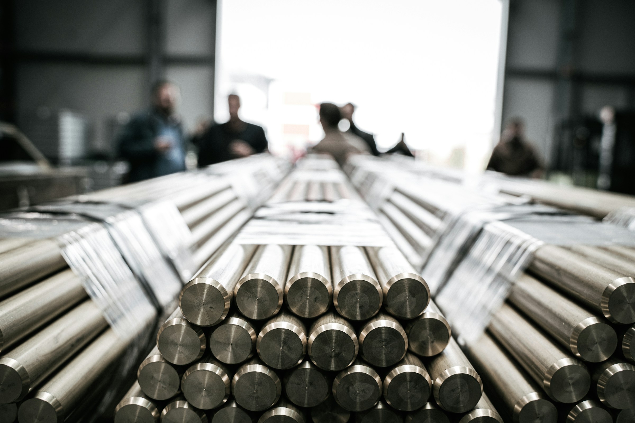
A rod reduces this problem to a single direction: we can move along its length, determine how much each short piece contributes, and combine those contributions. Consider a 2-meter metal rod that is thicker at one end than the other. How might its changing thickness affect its total mass?
The rod's linear density tells us how much mass is packed into each meter of length. For a rod with constant linear density, \[\text{mass}=\text{density}\times\text{length}.\]
For example, if the rod has linear density of \( 2 \) kg/m, its total mass would be kg.
For our rod, though, the density changes as we move from one end to the other. Let \( x \) be the distance in meters from the left end. At position \( x \), suppose the density is
\[\rho(x)=1+x\qquad(0\le x\le2),\]
in kilograms per meter. The Greek letter \( \rho \), pronounced “rho,” is often used for density. A single density can't give the exact mass of the whole rod, but we can use the density function to find an underestimate and an overestimate.
The minimum density along the rod is kg/m. If the entire \( 2 \) m rod had this minimum density, its mass would be kg. The actual density is never smaller, so this is a lower estimate for the rod's mass.
The same reasoning in the other direction gives an upper estimate. The maximum density is kg/m; if the entire rod had this maximum density, its mass would be kg. The actual density is never larger, so the rod can't have more than this much mass.
We now know that the rod's mass lies between \( 2 \) kg and \( 6 \) kg. This range is broad because each estimate uses one density for the entire rod, even though the density changes from one end to the other.
Instead, divide the rod into four pieces, each \( 0.5 \) m long. The density varies less within one short piece than it does across the whole rod, so the smallest and largest densities on each piece should give closer mass estimates. Since the density is increasing, those values occur at the piece's left and right endpoints.
Between \( x=0 \) and \( x=0.5 \), the length is m, while the density of that piece is at least kg/m and at most kg/m. This means that the mass of this first piece of the rod must be at least kg and at most kg.
We can repeat this calculation for the other three pieces of the rod:
| Piece (m) | Density (kg/m) | Mass estimate (kg) |
|---|---|---|
| \( 0\le x\le 0.5 \) | \( 1\le\rho\le 1.5 \) |
\( 0.5\le m\le0.75 \) |
| \( 0.5\le x\le 1 \) | \( 1.5\le\rho\le 2 \) | \( \le m\le \) |
| \( 1\le x\le 1.5 \) | \( 2\le\rho\le2.5 \) | \( \le m\le \) |
| \( 1.5\le x\le 2 \) | \( 2.5\le\rho\le 3 \) | \( \le m\le \) |
Then the total mass of the rod is the sum of the four smaller masses. Adding the four lower contributions gives a lower estimate of kg; adding the four upper contributions gives an upper estimate of kg. That's a much tighter range and gives us a better idea of what the actual mass might be.
Graphing density against position turns each mass estimate into an area. A rectangle's width is the length of one piece in meters, and its height is an assigned density in kilograms per meter. Its area has units of kilograms, so it represents the estimated mass of that piece. Adding the four rectangle areas gives the mass estimates we just found.
We can get a better approximation by cutting the rod into eight narrower pieces, represented by eight narrower rectangles. Their stair-step edges stay closer to the density graph, leaving less space between the lower and upper approximations.
If we add the areas of these rectangles, each of which has a width of m, the lower and upper bounds for the rod's mass become \( 3.75 \) kg and \( 4.25 \) kg. The gap between the bounds has changed from 1 kg to kg. With more, thinner pieces, each assigned density represents its piece more closely, and the lower and upper estimates squeeze toward the same mass.
We can continue increasing the number of rectangles. As their widths shrink, both collections of rectangles come to resemble the same region beneath the density graph.
Number of pieces:
At 100 pieces, the lower and upper estimates are \( 3.98 \) kg and \( 4.02 \) kg. The two staircases are almost impossible to tell apart from the region beneath the graph, although a small gap remains.
Smaller subdivisions give us better estimates of the rod's mass, but the calculations become more tedious, and no finite subdivision makes the density perfectly constant on every piece. We can always cut the rod again. The pattern suggests the same infinitesimal transition we used when we zoomed infinitely close to a curve: what if we continued subdividing the rod into infinitely many infinitesimal pieces? Each piece would then be thinner than any finite length we could measure, so its density could be treated as constant at that location.
The process of splitting something into infinitely many infinitesimal pieces and then adding them back up to get the whole is called integration.
Let's focus on one such piece at position \( x \). Its infinitesimal length is \( \dd{x} \), and its density is \( \rho(x) \). Since mass equals density times length, the piece has infinitesimal mass
\[\begin{aligned}\dd{m}&=\rho(x)\dd{x}\\ &=(1+x)\dd{x}\text.\end{aligned}\]
The symbol \( \dd{m} \) represents the mass of one infinitesimal piece.
To find the mass of the whole rod, we need to collect all of these infinitesimal masses, beginning at \( x=0 \) and continuing to \( x=2 \).
We write this new operation as
\[\begin{aligned}m&=\int_0^2\rho(x)\dd{x}\\ &=\int_0^2(1+x)\dd{x}\text.\end{aligned}\]
We call this expression an integral. The stretched-out letter S (\( \int \)) says that we're Summing infinitely many infinitesimal contributions. The \( 0 \) and \( 2 \) tell us where along the rod those contributions begin and end. Inside the integral, \( \rho(x)\dd{x} \) is the mass \( \dd{m} \) contributed by one infinitesimal piece.
The units multiply as we would expect: \( (\text{kg}/\text{m})\cdot\text{m}= \). Therefore, this integral represents the .
Back on the graph, the lower and upper staircases meet the density line when the pieces become infinitesimal. The whole region beneath the line represents the accumulated mass. For this linear density, that region is a trapezoid.
We can find the trapezoid's area using familiar geometry by splitting it along the dashed line. The part below the line is a rectangle of width \( 2 \) and height \( 1 \), while the part above it is a triangle with base \( 2 \) and height \( 2 \). Adding these areas gives us the value of our integral:
\(\displaystyle \int_0^2(1+x)\dd{x}=\)\(\displaystyle \text.\)
The horizontal units on our graph are meters and the vertical units are kilograms per meter, so this graphical area represents \( 4 \) kg of mass. It lies between every pair of lower and upper estimates we found.
Differentiation and integration are the two central tools of calculus. So far, we've used differentiation to understand change. In the next part of our study, we'll develop integration as a way to describe, calculate, and use accumulations.
From pieces to a whole
Many problems can be solved by breaking a whole into pieces, figuring out how much comes from each piece, and adding those amounts. When the amount changes from place to place, one value may not describe a large piece very well; in that case, narrower pieces usually give us a better estimate.
To describe this strategy mathematically, we'll use the word density in a broad sense. A density function \( f(x) \) tells us how much of some quantity is packed into one unit of \( x \) near the input \( x \). It might describe actual mass density, but the same idea can describe how other quantities are distributed.
Once we know the density, we can estimate the contribution from each piece. If one finite piece has width \( \Delta x \) and \( x \) is an input within it, then \( f(x)\Delta x \) estimates how much comes from that piece. Adding one term for every piece gives an estimate of the whole:
\[\text{total}\approx\sum f(x)\Delta x.\]
In this compact notation, the symbol \( \sum \) is the Greek letter "S" (called sigma), and it means to add (or Sum) one term for each piece. As we move from piece to piece, \( x \) is an input chosen within the current piece and \( \Delta x \) is that piece's width. The pieces don't have to be the same size; \( \Delta x \) means the width of whichever piece we're looking at.
The rod from Explore gives this broad idea of density a familiar physical meaning. On one piece of the rod, \( \rho(x) \) measures mass per unit length, so \( \rho(x)\Delta x \) estimates the piece's mass. Using the least density on each piece gives a lower sum, while using the greatest gives an upper sum. The actual mass lies somewhere between these sums.
The definite integral
A finite sum gives us a practical way to estimate an accumulation, but one density value still stands in for a whole piece of finite width. To describe the exact total, we use the same transition as in differentiation: we let those finite pieces become infinitesimal.
In Section 1.2, a finite change \( \Delta x \) became an infinitesimal change \( \dd{x} \) when we zoomed infinitely close. Here, the finite contribution \( f(x)\Delta x \) becomes the infinitesimal contribution \( f(x)\dd{x} \), and we collect all of those contributions across the interval. The change appears directly in the notation:
\[\text{total}\approx\sum f(x)\Delta x \qquad\longrightarrow\qquad \text{total}=\int_a^b f(x)\dd{x}.\]
The new symbol marks the transition from an estimated finite sum to an exact accumulation. The expression on the right is called a definite integral.
The notation keeps the structure of the finite sum visible: the sum symbol \( \sum \) becomes the integral symbol \( \int \), which is still an s for “Sum,” while the finite width \( \Delta x \) becomes the infinitesimal width \( \dd{x} \). At the same time, the approximation becomes an exact accumulation, and the bounds \( a \) and \( b \) tell us where the pieces start and stop.
Integrals and area
The integral notation describes an exact accumulation, while the graph gives us a geometric way to see the same process. In Explore, each estimated mass became a rectangle with height \( f(x) \) and width \( \Delta x \), so its area represented one finite contribution. When the widths become infinitesimal, these rectangles fill the region between a nonnegative graph and the horizontal axis, and the integral is represented by the area of that region.
If the region is a familiar geometric shape, its area gives the exact value of the integral. What that area means, however, depends on the quantities and units shown on the axes, and this is where the broad meaning of density becomes useful.
When the horizontal input is time, we often call the integrand a rate rather than a density. The underlying idea is the same: the integrand tells us how much of a quantity there is per unit of input. A rate \( q(t) \) tells us how much is happening per unit of time near \( t \), so \( q(t)\Delta t \) estimates how much happens during a short time interval and the integral adds those amounts over time.
The area interpretation doesn't depend on having a physical density or a rate. It can also evaluate an integral directly whenever the graph encloses a familiar geometric shape.
The rod, the flowing water, and the quarter-circle all use the same picture: the integrand gives the height, the differential gives an infinitesimal width, and the integral gives the total area. In the rod and water examples, that area represents a physical accumulation because the vertical quantity is measured per unit of the horizontal quantity. For the quarter-circle, it is ordinary geometric area.
This is what makes the integral so useful. A function describes what is happening near each input, and the integral brings all of those local contributions together into one total over an interval. The labels and units on the axes tell us what that total means.
A 2 m rod has density \( \rho(x)=2+x^2 \) kg/m.
Using four equal pieces, the left-end estimate is kg and the right-end estimate is kg.
Solution
Each piece is 0.5 m long. The left estimate is \( 0.5(2+2.25+3+4.25)=5.75 \) kg; the right estimate is \( 0.5(2.25+3+4.25+6)=7.75 \) kg.
Explain why these estimates bound the mass.
Solution
The density increases throughout the rod, so every left-end density is a minimum on its piece and every right-end density is a maximum. This gives \( 5.75\le m\le7.75 \) kg. Each contribution has units \( (\text{kg}/\text{m})\cdot\text{m}=\text{kg} \).
A cable has the following density measurements. Density decreases throughout each interval.
\( x \) (m) 0 1 3 4 \( \rho(x) \) (kg/m) 6 5 3 2 Using these three intervals, a lower mass bound is kg and an upper bound is kg.
Solution
The lengths are 1, 2, and 1 m. Right endpoints give the lower bound \( 5(1)+3(2)+2(1)=13 \) kg. Left endpoints give the upper bound \( 6(1)+5(2)+3(1)=19 \) kg. Equal weighting would misrepresent the 2 m middle piece.
Use geometry to find each integral. The graph of each integrand lies on or above the horizontal axis over the interval shown.
\( \displaystyle \int_0^{${rectangle_width}}${rectangle_height}\dd{x}= \)
Solution
The constant integrand forms a rectangle with width \( ${rectangle_width} \) and height \( ${rectangle_height} \). Therefore,
\[\int_0^{${rectangle_width}}${rectangle_height}\dd{x}=(${rectangle_width})(${rectangle_height})=${rectangle_area}.\]
\( \displaystyle \int_0^{${triangle_width}}${triangle_slope}x\dd{x}= \)
Solution
The line rises from \( 0 \) to \( ${triangle_height} \), so the region is a triangle with base \( ${triangle_width} \) and height \( ${triangle_height} \). Hence,
\[\int_0^{${triangle_width}}${triangle_slope}x\dd{x}=\frac12(${triangle_width})(${triangle_height})=${triangle_area}.\]
\( \displaystyle \int_0^{${trapezoid_width}}(${trapezoid_left_height}-${trapezoid_slope}x)\dd{x}= \)
Solution
The line decreases from height \( ${trapezoid_left_height} \) to height \( ${trapezoid_right_height} \), which remains positive. The region is a trapezoid of width \( ${trapezoid_width} \), so
\[\int_0^{${trapezoid_width}}(${trapezoid_left_height}-${trapezoid_slope}x)\dd{x}=\frac12(${trapezoid_left_height}+${trapezoid_right_height})(${trapezoid_width})=${trapezoid_area}.\]
The graph of \( f(x)=${graph_line} \) has a shaded region between the curve and the horizontal axis. Write a definite integral whose value equals the shaded area.
The shaded region extends from \( x=${graph_left} \) to \( x=${graph_right} \). In the answer box, type int to insert an integral. Enter the lower bound, press the up arrow for the upper bound, and then press the right arrow to enter the integrand and differential.
Solution
The horizontal bounds of the shaded region are \( ${graph_left} \) and \( ${graph_right} \), and its height is \( f(x)=${graph_line} \). Therefore, the area is represented by
\[\int_{${graph_left}}^{${graph_right}}(${graph_line})\dd{x}.\]
Along a \( ${road_length} \) km stretch of road, the tree density is modeled by \( t(x)=${tree_start_density}+${tree_density_slope}x \) trees per kilometer, where \( x \) is the distance in kilometers from the beginning of the stretch.
Explain what \( t(x)\Delta x \) represents.
Solution
The value \( t(x) \) gives trees per kilometer near position \( x \). Multiplying by a short length \( \Delta x \) estimates the number of trees along that piece of road.
The model predicts a total of trees along the stretch.
Solution
The density rises from \( ${tree_start_density} \) to \( ${tree_end_density} \) trees per kilometer, so the region beneath its graph is a trapezoid. Therefore,
\[\int_0^{${road_length}}(${tree_start_density}+${tree_density_slope}x)\dd{x}=\frac12(${tree_start_density}+${tree_end_density})(${road_length})=${tree_total}\text{ trees}.\]
Two rods have the same length and the same densities at both ends. Must their masses be equal? Support your answer with two possible density profiles.
Solution
No. On a 1 m rod, the densities \( \rho_1(x)=1 \) and \( \rho_2(x)=1+x(1-x) \) kg/m both equal 1 at the ends. The second is greater everywhere in the interior, so its interior pieces contribute more mass and its total mass is greater. Endpoint measurements alone don't describe the whole accumulation.